Running Difwrap
To start difwrap, first change to the directory where your data is, then
type difwrap. Difwrap will start up the GUI, and then start
a Difmap session. When this is complete, the main menu window will
appear:
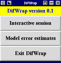
Figure 2.1: the Difwrap main menu.
|
Choosing ``Interactive session'' will allow you to interact with Difmap
as normal. To return to Difwrap, type <Control>-W (i.e.
hold down the [Control] key and press the W key).
Choosing ``Model error estimates'' will start up the error analysis
GUI as described in Section 2.2 while
choosing ``Exit DifWrap'' will exit the program.
How to use the error analysis
GUI
Below are step-by-step instructions for carrying out a model component
error analysis.
-
1.
-
After starting Difwrap, choose ``Interactive session'' from the
main menu and carry obtain the best fit model to your data as normal.
-
2.
-
Type <Control>-W to return to the main menu and select ``Model
error estimates''. You will be presented with window (Figure 2.2)
which you can use to choose the model component of interest, the range
of values to test and the error fitting method.
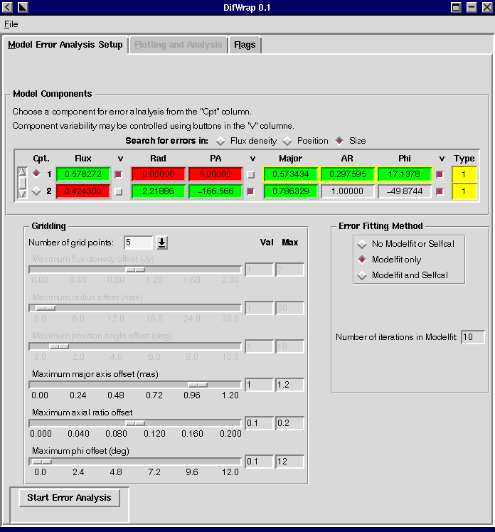
Figure 2.2: Model error analysis setup window.
|
-
3.
-
Model Components. Near the top of the window is a list of your model
components. Those parameters with a green background you have selected
as variable while those with a red background are non-variable. You can
alter the variability state by clicking on the square buttons in the columns
marked by a ``v''. Select the model component of interest by clicking on
a button in the left-hand column. Select the parameter of interest (either
flux density, Position or Size) from the buttons above the list of model
components. In figure 2.3, the size
of component number 1 has been selected.
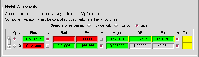
Figure 2.3: Model component selection.
|
-
4.
-
Gridding. For each value that describes a parameter, the range and
number of values you wish to test must be selected. This is done through
the Gridding section of the window. The number of grid points to
be sampled for each range of values is selected together with the maximum
offset of each parameter. This can be done by moving the horizontal sliders
to the desired position or by typing in the desired values manually in
the boxes in the Val column. For example, in Figure 2.4
5 grid points have been requested in each dimension2.1
and the range of values
 mas in major axis,
  in axial ratio and
  in major axis position angle from the best fit will be trialed.
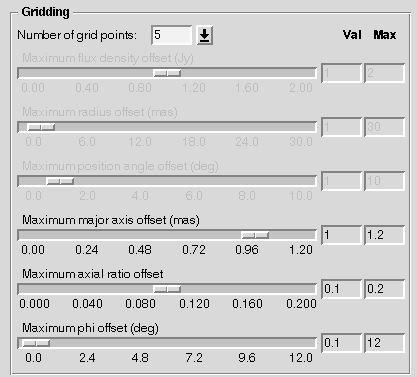
Figure 2.4: Gridding selection.
|
-
5.
-
Error Fitting Method. Lastly, the error fitting method (as described
above) must be selected together with the number of modelfit iterations.
For example, in Figure 2.5 the ``Modelfit
only'' method has been chosen with 10 iterations in modelfit.2.2
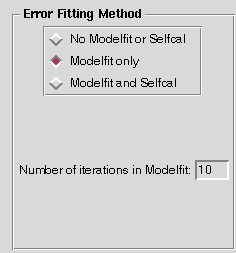
Figure 2.5: Error fitting method selection.
|
-
6.
-
Once this setup page has been configured, the analysis is started by pressing
the Start Error Analysis button.
-
7.
-
A Status window will appear providing an indication of the progress of
the modelfitting (Figure 2.6).
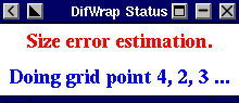
Figure 2.6: Error fitting method selection.
|
-
8.
-
When Difwrap has finished sending commands to Difmap, a new
window will appear from which you can choose how the results are to be
presented (Figure 2.7). The goodness
of fit (either rms or Chi-squared) of each trial model can be plotted as
a function of the trial values. The user can select a grid point and Difwrap
will ask Difmap to display the corresponding model with the data
using vplot, radplot or projplot. Select the
Difmap command you would like executed from the ``inspect data using''
box and how the goodness of fit results are to be shown from the ``plotting''
box.
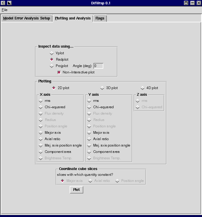
Figure 2.7: Plotting and Analysis window.
|
-
9.
-
Figure 2.8 shows Chi-squared as a
function of Flux density for a 9-point grid analysis to estimate the error
in flux density of a model component. Clicking on a point with the left
mouse button will result in the corresponding model to be displayed with
the data. That point will then be surrounded by an orange circle to indicate
that the point has been inspected. If the user decides that the model corresponding
to that point is a good representation of the data, clicking the middle
mouse button over it will change its colour from red to green, indicating
acceptance. In this example, the central three grid points have been deemed
acceptable while the others are unacceptable. Clicking the right mouse
button in the window returns the user to the plotting window (Figure 2.7)
and the estimated flux density errors are displayed in the message window
(Figure 2.9). Difwrap estimates
the errors by taking the most extreme accepted points. The contents of
this window can be edited and saved or printed out using the ``Save as''
and ``Print'' commands respectively under the ``File'' menu.
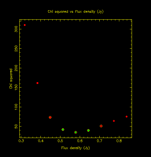
Figure 2.8: A plot of modelfitting results.
|
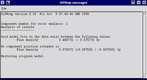
Figure 2.9: The messages window showing results of a flux
density error analysis.
|
-
10.
-
Further plotting may be done, or a new error analysis session may be started.
Footnotes
-
... dimension2.1
-
i.e. In this case there are three dimensions to be sampled: major
axis, axial ratio and major axis position angle. There are 5 grid points
to be sampled per dimension, resulting in
 points to be sampled.
-
... modelfit.2.2
-
i.e. The command modelfit 10 will be executed in Difmap.
Jim Lovell
1998-10-12